1. IntroductionLiDAR point-cloud data contain high-resolution information about the earth’s surface – terrain, hardscape, and vegetation. These data can be applied to virtually any field of study and are a useful addition to your GIS analysis. The purpose of this workshop is to gain basic skills in loading, viewing, manipulating, and processing LiDAR data in ArcGIS Pro. By the end of this workshop, you will be able to:
Downloading the Workshop Data
Below are the steps to extract the workshop material: 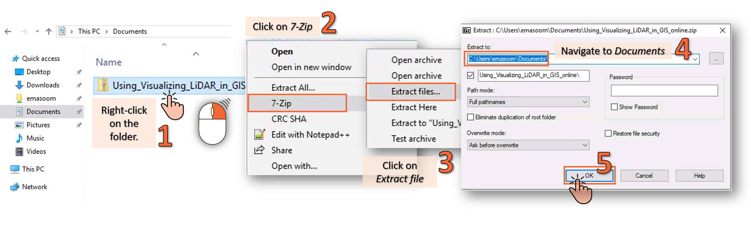 Go to the Start menu and open ArcGIS Pro and sign in using your Clemson ID.  Click on Open another project, navigate to the workshop folder, click on Using_Visualizing_LiDAR_in_GIS.aprx within the folder you copied.  Enabling the 3D Analyst ExtensionThe tools for working with LiDAR are part of the 3D Analyst extension. We are going to make sure that the necessary extensions are enabled. Click in the upper-left corner on Project > Licensing > Configure your licensing options. Check the boxes next to Spatial Analyst and 3D Analyst if not already enabled. Click OK and then the back arrow to return to the Map view.What is LiDAR? LiDAR, which stands for Light Detection and Ranging, is a remote sensing method that uses light in the form of a pulsed laser to measure ranges (variable distances) to the Earth. These light pulses—combined with other data recorded by the airborne system— generate precise, three-dimensional information about the shape of the Earth and its surface characteristics. How is LiDAR Collected?Sensors are mounted to aircraft, unmanned aerial vehicles (UAV), railways, passenger vehicles, tripods, boats and spacecraft… LiDAR scanner mounted to aircraft emits laser pulses which scan the ground.Ranging gives distance from scanner to reflecting object. GPS (Geographic Positioning System) locates the scanner’s position coordinates. IMU (Inertial Measurement Unit) gives orientation of the scanner. Scanners can collect from a hundreds to over a million of points per second. Creating a LAS dataset An LAS file is an industry-standard binary format for storing airborne lidar data. ArcGIS Pro can use the LAS files directly, but often these come as a collection of adjacent files. To work with a collection of LAS files you create a LAS dataset which stores reference to one or more LAS files on disk, as well as to additional surface features. The LAS dataset allows you to examine LAS files easily and quickly obtain detailed statistics and inspect the aerial coverage of the LiDAR data contained in the LAS files. Let’s start by looking at the LAS files we will be working with.
Right-click on the first file and open the Properties. On the General tab, take a look at the XY Linear Unit and Z Unit. Notice that XY Linear is Not Available.  Select the Coordinate System tab. Notice that the coordinate system is geographic coordinates (i.e. longitude and latitude). As a growing GIS user, you know that working in projected coordinates are much better for analysis. In particular, LiDAR data stored in geographic coordinates will cause problems with display in ArcGIS. We will reproject the files in a few steps. First, let’s create the LAS Dataset to work with this group of LAS files. In the Catalog pane, right-click on the LAS_Files folder and select New > LAS Dataset. The item will be created in the folder. Rename it Clemson_Campus.lasd. Right-click on the new LAS Dataset and select Properties > LAS Files tab. Click Add Files…. Navigate to the LAS_Files folder and select the following files: 20110319_SC_PickensCo_2011_000034.las 20110319_SC_PickensCo_2011_000035.las 20110319_SC_PickensCo_2011_000040.las 20110319_SC_PickensCo_2011_000041.las 20110319_SC_PickensCo_2011_000065.las 20110319_SC_PickensCo_2011_000071.las  Click Open. Next, go to the Statistics tab and click the Calculate button to generate statistics. Take a minute to look at the information calculated. On the General tab, check the box to Store relative path names to data sources. Click OK.  On the Analysis tab, select Tools. The Geoprocessing pane extract las opens. In the Search bar, type Extract LAS and hit enter. Click to open the tool and enter these parameters: - Input LAS Dataset: Browse to Clemson_Campus.lasd - Target folder: LAS_Files - Output LAS Dataset: Give the name Clemson_Campus_Projected.lasd Click LAS File Options to expand the menu. Set Output File Name Suffix to _proj At the top of the tool, click Environments. Click the Select Coordinate System button. Set the Output Coordinate System to NAD 1983 2011 StatePlane South Carolina FIPS 3900 (found in Projected Coordinate System > State Plane > NAD 1983 (2011) (Meters)). Click Run.  The newly created dataset is added to the map and will show the extent of each file as a red box. Look in the Contents pane and notice that the Data percentage is currently 0. (You may need to expand the layer). At this scale, there are too many points for the software to render. Zoom in to the map and at a certain scale, you will see the pointsdisplay. Switch the basemap to Imagery and take a look at differentareas of the map. In particular, look around Lake Hartwell, near Death ValleyStadium, and zoomed in very closely (1:300 or higher). What are yourobservations about the point cloud data?   Click on the Clemson_Campus_Projected.lasd inthe Contents pane, then go to Appearance. Dragthe Density Min slider over to Min, then to Max. Change the Display Limit to 5000000 (5 million). Notice how the Datapercentage changes in the Contents panel. The softwarewill randomly thin the point cloud to speed up display. It does not affect theunderlying data. 3. LiDAR Returns, Classification, and Attributes (video link)
Zoom inclose enough to clearly see distinct points (about 1:200 scale). From the Map tab, select the Measure tool. Click on a point to start themeasurement, then double-click on another point to finish. Measure the pointspacing for a few points. Q. What do you find for the minimum and maximum spacing?Q.What is your estimate of the average spacing? Q. What might affect the spacing between points? Close the Measure Distance tool window. In the Catalog pane, click onProject to see the Folders, right-click on Clemson_Campus.lasdand open the Properties. Go to theLAS Files tab. Q. What point spacings are listed in the LAS Dataset properties?? LiDAR ReturnsWhen the LiDAR data are collected, the instrument may record multiplereflections, called returns, andlabels each point with the return number. The first return from a specific location will be a reflection from theupper-most feature, such as the top of a tree. Successive returns (second,third, and fourth) will be from lower elevations than the first return. Ifthere are no above-ground objects, then the first return will be a reflectionfrom the ground surface. In some situations, such as very dense tree canopies,only the first return may be recorded and ground- return points will be sparse. Classifying LiDAR data
LiDAR StatisticsWhen we created the Clemson_Campus.lasd LAS Dataset, we calculated the Statistics, which give us detailed information about point spacing as well as the percentage of points falling into certain classification codes or return types. Statistics are important to calculate because point filters will not work properly without them! Let’s review the statistics in more detail. With theProperties still open, select the Statistics tab. Q. What are the supplied classification codes? Q. How might the points pacing affect the usefulness of our LiDARdata? Close the Las DatasetProperties window. 4. Visualization and Symbology (video link)ArcGIS can draw your LiDAR point clouds in a variety of ways. When LiDAR data are first added to a map or scene view, the points are assigned a color according to elevation and broken into classes.The software can also interpret the LASfile classifications and return types and quickly visualize the LiDAR pointsbased on return number or classification code from the Appearance tab in the LASDataset Layer group. Click on LAS Points dropdown and click on All Points. Zoom in and out to explore the map. Do the same process with Ground, Non-Ground, and First Return Points.  The data can also be drawn as a surface (a triangular irregular network,or TIN) which represents either elevation, slope, or aspect of the surface. On the Appearance tab, select Symbology.Try dragging the Symbol scale slider. Click on Symbology on the Appearance tab and select Class. Pan around the map area.
 Q. What class codes do you see present in the data? Q. What class codes do you see present in the data?Change the Symbology to Return and pan around the map area. Q. Where are locations with 4 returns? (Hint: change the color of the 4th return if needed).Q. Why are the 4th returns found in that location?
Q. What sort of patternsdo you notice about the distribution of intensity values?  Symbolizing LiDAR data using a surface-based renderer The Surface display illustrates the points as a TIN surface. Try changing thesymbology to an Elevation surface display.Then, experiment with changing the view to Slope, and Aspect.  You can apply different filters, whichwork on the classification and/or return, similar to a selection on vectordata. Change back to a surface showing Elevation.In the Filters group, click LAS Points tosee the dropdown and select Ground. View the result on the map. 5. Viewing LiDAR in a 3D Scene (video link)With ArcGIS Pro, you can create and share 3D visualizations that engage viewers and support informed decision making. In this section, we will get familiar with the ArcGIS Pro 3D environment and learn techniques to create and enhance 3D scenes. Creating a sceneAs we mentioned, ArcGIS Pro has excellent 3D visualization capabilities. We can easily convert a map view to a scene view. Let’s convert our map and look at our point cloud in more detail. Set the Symbology back to Points showing Elevation. Then, go to the View tab and select Convert > To Local Scene. Use the Explore tool to move around the scene. Get comfortable zooming in and out and rotating the view.  Profile view In a Scene view, you are able to view 2D cross-sectional slices of the data. In the LAS Dataset Layer group and Classification tab, select the Create option in the Profile Viewing group. Click on a point somewhere to the north of the stadium. Then click on another point somewhere south of the stadium, and the view will change to show a profile of points along that line. Using the Measure tool, determine the height difference from the field level to the top of Death Valley stadium.  Q. How tall is the stadium? Are both sides equal in height? 3D visualization helps to clarify where the first, second, third, and fourth returns occur. Change the Symbology to Return and adjust the Color scheme as needed. Q. Where do you notice multiple returns happening in 3D space? Save the project.  6. Classifying and Reclassifying the Point Cloud (video link) Raw data from a LiDAR scanner does not have any classification applied. Classification codes are added to each point using a combination of processing tools and manual classification. There are several tools for classifying point cloud data in ArcGIS Pro. One example is using vector data to apply class codes by overlay. For example, we have building footprints for Clemson and can overlay these on the point cloud. Points within the footprints will be assigned the building class code. There will be discrepancies between which buildings are present in the LiDAR data from 2011 and building footprints from 2016, but most of the classification will be correct. In the Catalog pane, go to Using_Visualizing_LiDAR_in_GIS.gdb and expand the geodatabase. Add the layer titled Buildings_CU_2016_2D. Click on the Clemson_Campus_Projected.lasd in the Contents panel. In the LAS Dataset Layer group and Classification tab, click on Feature Proximity and 2D Proximity. Set the following parameters for the tool:  When the tool completes, remove the LAS dataset from the scene and add it once again from the Catalog pane. View the result using a Classification symbology. In some cases, you may have LiDAR data without any classification codes. In ArcGIS Pro, there are tools for classifying points representing the ground surface, buildings, and vegetation. Let’s try it out. First, we will use a geoprocessing tool to perform automatic classification of ground points. In a nutshell, the tool will identify a subset of points that are reasonably flat and smooth without spikes (trees) or big discontinuous changes in elevation (rooftops). From the LAS_Files folder, add the 20110319_SC_PickensCo_2011_000041_NOCLASS.las to the scene from the Catalog pane. Click on it in the Contents pane and in the Classification group, click on Automated Classification> Classify Ground. Leave the Ground Detection Method set to Standard Classification. This will allow for some undulation in topography. Click Run.  When the tool finishes, remove the LAS file from the scene and add it once again. Change the Symbology to show Classification and apply the Ground filter. View the result, and then remove the Ground filter.
Now let’s classify buildings using the automated tool. Select 20110319_SC_PickensCo_2011_000041_NOCLASS.las in the Contents pane, go to Classification > Automated Classification > Classify Buildings. Accept the default options and click Run.
When finished, turn off the layer and turn on Clemson_Campus_Projected.lasd.  LiDAR data can have very small point spacings (sub-meter to cm scale!) and thus can represent topography, buildings, roads, forests, and other features with excellent detail. These high- resolution data can be used to create raster elevation models with very small grid spacing. Many spatial analysis tools and workflows don’t yet work directly on point-cloud data but will work on rasters derived from LiDAR. Let’s use our Clemson_Campus_Projected.lasd LiDAR dataset to create high-resolution elevation rasters. We will use only the ground-classified returns to construct a digital elevation model (DEM) and then the first returns to create a model of the highest elevations, called a digital surface model (DSM).  We will first create the DEM from Clemson_Campus_Projected.lasd using the ground-classified returns. Click on Clemson_Campus_Projected.lasd, then on the LAS Dataset Layer > Appearance tab, click LAS Points > Ground to filter the point cloud. This filtering works much like a selection on a vector data set. Geoprocessing tools run on the point cloud will use only the points we select. In the Geoprocessing pane, search for the LAS Dataset to Raster tool. Click on it to open. Set the following tool parameters: Input LAS Dataset: Clemson_Campus_Projected.lasd Output Raster: Clemson_DEM in the project geodatabase Value Field: Elevation Sampling Value: 1 Leave the other parameters with the defaults, then click Run. When the tool completes, the elevation raster will be added to the view. Turn off layers, as necessary, to see the output. Q: What are the minimum/maximum elevations? Q. What do you notice about the western edge of campus right next to Lake Hartwell? Q. What are your observations or remarks on the created DEM?  Next, we will create the DSM using first returns. From the LAS Dataset Layer > Appearance tab, click LAS Points > First Return Points. Open the Geoprocessing pane again to the LAS Dataset to Raster tool. Use the same parameters as before, but change the name of the output raster: Input LAS Dataset: Clemson_Campus_Projected.lasd Output Raster: Clemson_DSM in the project geodatabase Value Field: Elevation Sampling Value: 1 Leave the other parameters with the defaults, then click Run. Q. What are the minimum/maximum elevations?Q. What are your observations on the DSM? Q. How might the DSM be used differently from the DEM? 8. LiDAR ApplicationsThe following activities demonstrate applications of LiDAR data through scenarios in which you, a GIS consultant, are asked to solve a problem or give a recommendation. We will use what we have learned about LiDAR data to demonstrate why LiDAR data are so useful for geospatial analysis. A viewshed is the geographic area visible from a specific location, either a point or a line. Finding which areas are visible, or not visible, is important when you are locating a feature which needs lots of visibility, such as a fire tower, or in placing unattractive features out of sight, such as a parking lot. Scenario: A large flag is to be raised to commemorate Clemson’s 125th anniversary. The goal is for the flag to be visible across as much of campus and the immediate surroundings as possible, but needs to be placed on an existing building. It will ideally be visible from the three primary highways leading to Clemson: highway 123 from the west, highway 93 from the east, and highway 76/28 from the south. Where should it be placed to meet most, if not all, of these criteria? Can it be done from a single location? Where would you try first? Solution: We can do a line-of-sight analysis with our point cloud to evaluate whether some feature is visible from another point. Performing a viewshed analysis using our DSM of Clemson and the proposed location(s) will show us what regions are visible. From this, we can determine whether the goal is feasible using our proposed locations. To start, we will use the Line of Sight tool to evaluate whether Tillman Hall can be seen from the three highways leading to campus. From the Using_Visualizing_LiDAR_in_GIS geodatabase, add the Sight_Lines feature class, which contains 3D line features connecting each highway to the top-most point representing Tillman Hall. Click on the Clemson_Campus_Projected.lasd in the Content pane and then the Data tab. Click Visibility > Line of Sight to open the tool. Set the Sight_Lines as the Input Line Features, and save the output as Tillman_LOS. Click Run and then view the result. The lines are split into segments, with a green color indicating a visible segment from the observation point and red color indicating not visible. .png)  Next, let’s evaluate from the viewshed method to find all the areas visible from the top of Tillman Hall. In the Geoprocessing window, search for Viewshed (Spatial Analyst) and click to open the tool. Set the following parameters: Input Raster: Clemson_DSM Input Observer Features: click the pencil icon and then click Points to draw in an observer feature. Navigate to Tillman Hall and draw in a point as near as you can to the top of Tillman Hall, using the LiDAR points as a guide. Output raster: Tillman_viewshed in the geodatabase. Click Run and then view the result, which will be symbolized by visibility. Q. Which areas have excellent visibility of Tillman Hall? Q. What areas are obvious obstructions to visibility?
 Locating a Solar Panel Array Locating a Solar Panel ArrayScenario: The University wants to build an array of solar panels on a building rooftop on campus and needs to know which buildings would be best suited for this purpose. Solution: We can calculate the insolation (solar radiation) received on each of the buildings using the DSM, which gives us the elevation as well as the aspect (direction) and slope of the buildings. The LiDAR data provide high-resolution elevation information to calculate incoming solar radiation varies across individual rooftops, enabling us to optimize the placement of solar panels. To begin our analysis, insert a new Map view (go to Insert > New Map > New Map). Add the Clemson_DSM raster and the Buildings_CU_2016_2D dataset to the map. Save your project. We will use the Area Solar Radiation tool to calculate incoming energy. We will calculate for a specific day – the winter solstice on December 21, to show the minimum amount of energy expected. This calculation is fairly intensive, so to speed things up, we will clip out our DSM to only those areas where we have buildings. In the Geoprocessing pane, search for and open the Extract by Mask tool. Use these tool parameters:
Input raster or feature mask data: Buildings_CU_2016_2D/Buildings_CU_2016_2D. Output raster: Bldgs_DSM Click Run. The output raster is clipped to only the locations of the building footprints. Next, search for and open the Area Solar Radiation (Spatial Analyst) tool in the Geoprocessing pane. Use the following parameters: Input raster: Bldgs_DSM. Notice that the Latitude value automatically populates. Output global radiation raster: Clemson_Solar_Rad in the geodatabase. Time configuration to Within day, and select day 355 (December 21). Explore the other parameters for the tool, then click Run. This may take a few minutes to process. The Clemson_Solar_Rad raster is added to the map showing the insolation received by building rooftops. Q. What are your thoughts on where the best locations for solar panels would be? The height of the tallest vegetation above ground level is termed the canopy height. Characterization of the canopy height in a forest is useful for studying forest succession, understanding the history of a forested site, monitoring logging and recovery, and in evaluating certain types of forest habitat. The canopy height can be determined by subtracting a ground- return DEM from a first-return DSM of the forest. Scenario: The Clemson Tiger-bird, avery rare creature, has been spotted south of the university in a forest tract adjacent to LakeHartwell. We have an LAS Dataset for this forest tract named Clemson_Forest.lasd.The animal only nests in smaller second-growth trees of 5-10 m height, and landmanagers want to identify areas of potential habitat for this unique animal intheir tract as well as a percentage of the area which may constitute habitat. Determining Canopy Height Using Rasters Hint 1: your first step is to create a DEM and DSM from our LiDAR dataset. Let’sinsert an additional Map view (go to Insert >New Map > New Map). Rename the Map to CanopyHeight. Add the Clemson_Forest.lasd tothe map. Save your project.
Hint 2: Use what you have learned to create a DEM and DSM from the Clemson_Forest.lasd file.Make the rasters with 1 m resolution andsave as integer rasters. Save the DEM as Forest_DEMand the DSM as Forest_DSM. Hint 3: In the Geoprocessingpane, search for the Minus (Spatial Analyst)tool Determining Canopy Height by Reclassifying the LAS Data You can add new classification codes to your LAS files based on their height. In this way, the points themselves can be quickly visualized using the tools in ArcGIS as well as processed a bit differently.Hint1: Inspect the source LAS file, the statistics, and note the current classes. Class 4 will represent our ideal tiger-bird habitat. Hint 1: Use the Classify LAS By Height (3D Analyst) tool.Q. What percentage of the Clemson_Forest_Reclass.lasd dataset is classified as MediumVegetation? Q. What advantages or drawbacks would this method have over the raster method? Other resources:
Congratulations! You now have the knowledge you need to incorporate LiDARinto your GIS work. |


